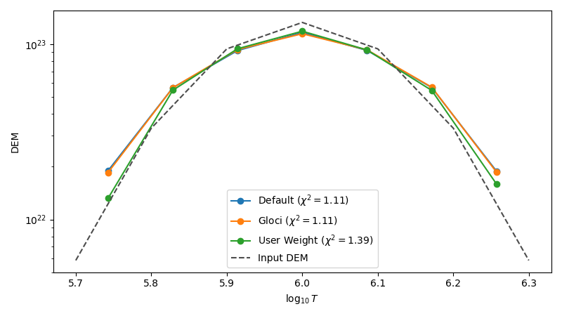
Compare Weighting Strategies

Compare the default self-normalized constraint, gloci, and a user-supplied weight. All three runs use the same synthetic data, so the only difference is how the weighting curve for the constraint is chosen. The point is to show how much the recovered DEM can move when that choice changes.

import matplotlib.pyplot as plt
import numpy as np

from demregpy import dn2dem
from demregpy.synthetic import synthesize_counts

This setup keeps the data fixed so the weighting choice is the only moving part. If the recovered curves stay close, this particular problem is not especially sensitive to the weighting scheme.

tresp_logt = np.linspace(5.7, 6.3, 7)
response_centers = np.array([5.75, 5.85, 5.95, 6.05, 6.15, 6.25])
trmatrix = np.zeros((tresp_logt.size, response_centers.size))
for i, center in enumerate(response_centers):
    trmatrix[:, i] = np.exp(-((tresp_logt - center) ** 2) / (2 * 0.08 ** 2))

root2pi = np.sqrt(2.0 * np.pi)
dem_model = (4e22 / (root2pi * 0.12)) * np.exp(-((tresp_logt - 6.0) ** 2) / (2 * 0.12 ** 2))
synthetic = synthesize_counts(dem_model, tresp_logt, trmatrix, error_fraction=0.1)

temps = 10 ** np.linspace(tresp_logt.min(), tresp_logt.max(), tresp_logt.size + 1)
mlogt = 0.5 * (np.log10(temps[:-1]) + np.log10(temps[1:]))
user_weight = 10 ** np.interp(mlogt, tresp_logt, np.log10(dem_model))
user_weight /= np.max(user_weight)

solutions = {
    "Default": dn2dem(
        synthetic.dn_in,
        synthetic.edn_in,
        trmatrix,
        tresp_logt,
        temps,
        nmu=50,
        warn=False,
    ),
    "Gloci": dn2dem(
        synthetic.dn_in,
        synthetic.edn_in,
        trmatrix,
        tresp_logt,
        temps,
        gloci=1,
        nmu=50,
        warn=False,
    ),
    "User Weight": dn2dem(
        synthetic.dn_in,
        synthetic.edn_in,
        trmatrix,
        tresp_logt,
        temps,
        dem_norm0=user_weight,
        nmu=50,
        warn=False,
    ),
}

for label, result in solutions.items():
    print(f"{label:>12s} chi-squared: {result[3]:.3f}")

    Default chi-squared: 1.106
      Gloci chi-squared: 1.115
User Weight chi-squared: 1.388

The useful question here is not which line looks nicest, but whether different weighting choices lead to materially different conclusions. If they do, the data quality, temperature coverage, and prior assumptions need more attention.

fig, ax = plt.subplots(figsize=(8, 4.5))
for label, result in solutions.items():
    ax.plot(mlogt, result[0], marker="o", label=f"{label} ($\\chi^2={result[3]:.2f}$)")

ax.plot(tresp_logt, dem_model, "--", color="0.3", label="Input DEM")
ax.set_xlabel(r"$\log_{10} T$")
ax.set_ylabel("DEM")
ax.set_yscale("log")
ax.legend()
fig.tight_layout()
plt.show()