Compare EMD-Like Modes

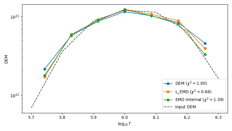
Compare the standard DEM inversion with the EMD-oriented options. This example uses one broader synthetic DEM so the effect of the different EMD-related options is easier to inspect. The main question is how much of the recovered structure comes from the data and how much comes from the chosen constraint.

import matplotlib.pyplot as plt
import numpy as np

from demregpy import dn2dem
from demregpy.synthetic import synthesize_counts

The input DEM has two overlapping components so the effect of the different constraint choices is easier to see. In practice this kind of comparison tells you how sensitive the recovered shape is to the form of the regularization.

tresp_logt = np.linspace(5.7, 6.3, 7)
response_centers = np.array([5.75, 5.85, 5.95, 6.05, 6.15, 6.25])
trmatrix = np.zeros((tresp_logt.size, response_centers.size))
for i, center in enumerate(response_centers):
    trmatrix[:, i] = np.exp(-((tresp_logt - center) ** 2) / (2 * 0.08 ** 2))

root2pi = np.sqrt(2.0 * np.pi)
dem_model = (
    (2.5e22 / (root2pi * 0.11)) * np.exp(-((tresp_logt - 5.95) ** 2) / (2 * 0.11 ** 2))
    + (2.0e22 / (root2pi * 0.10)) * np.exp(-((tresp_logt - 6.12) ** 2) / (2 * 0.10 ** 2))
)
synthetic = synthesize_counts(dem_model, tresp_logt, trmatrix, error_fraction=0.1)

temps = 10 ** np.linspace(tresp_logt.min(), tresp_logt.max(), tresp_logt.size + 1)
mlogt = 0.5 * (np.log10(temps[:-1]) + np.log10(temps[1:]))

solutions = {
    "DEM": dn2dem(
        synthetic.dn_in,
        synthetic.edn_in,
        trmatrix,
        tresp_logt,
        temps,
        nmu=50,
        warn=False,
    ),
    "L_EMD": dn2dem(
        synthetic.dn_in,
        synthetic.edn_in,
        trmatrix,
        tresp_logt,
        temps,
        l_emd=True,
        nmu=50,
        warn=False,
    ),
    "EMD Internal": dn2dem(
        synthetic.dn_in,
        synthetic.edn_in,
        trmatrix,
        tresp_logt,
        temps,
        emd_int=True,
        emd_ret=False,
        gloci=1,
        nmu=50,
        warn=False,
    ),
}

All three solutions are plotted against the same input curve. Large differences are not automatically bad, but they do mean the regularization choice is part of the scientific interpretation.

fig, ax = plt.subplots(figsize=(8, 4.5))
for label, result in solutions.items():
    ax.plot(mlogt, result[0], marker="o", label=f"{label} ($\\chi^2={result[3]:.2f}$)")

ax.plot(tresp_logt, dem_model, "--", color="0.3", label="Input DEM")
ax.set_xlabel(r"$\log_{10} T$")
ax.set_ylabel("DEM")
ax.set_yscale("log")
ax.legend()
fig.tight_layout()
plt.show()