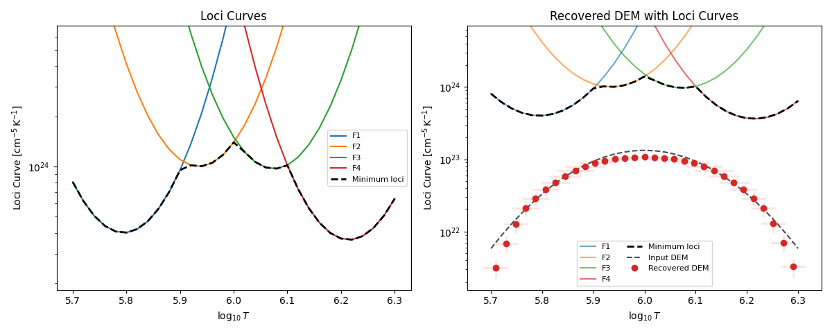
Plot Loci Curves

Plot filter loci curves and overlay them on a recovered DEM.

import matplotlib.pyplot as plt
import numpy as np

from demregpy import dn2dem
from demregpy.plotting import plot_dem, plot_loci_curves
from demregpy.synthetic import synthesize_counts

Loci curves are useful as an upper bound on the recovered DEM. The plotting helper uses the same bin-aware scaling as dn2dem by default, so the loci curves can be drawn on the same axes as a DEM.

tresp_logt = np.linspace(5.7, 6.3, 31)
response_centers = np.array([5.78, 5.92, 6.06, 6.20])
trmatrix = np.zeros((tresp_logt.size, response_centers.size))

for i, center in enumerate(response_centers):
    trmatrix[:, i] = np.exp(-((tresp_logt - center) ** 2) / (2 * 0.08 ** 2))

root2pi = np.sqrt(2.0 * np.pi)
dem_model = (4e22 / (root2pi * 0.12)) * np.exp(
    -((tresp_logt - 6.0) ** 2) / (2 * 0.12 ** 2)
)

synthetic = synthesize_counts(
    dem_model,
    tresp_logt,
    trmatrix,
    error_fraction=0.1,
)

temps = 10 ** np.linspace(tresp_logt.min(), tresp_logt.max(), tresp_logt.size + 1)
mlogt = 0.5 * (np.log10(temps[:-1]) + np.log10(temps[1:]))
dem, edem, elogt, chisq, dn_reg = dn2dem(
    synthetic.dn_in,
    synthetic.edn_in,
    trmatrix,
    tresp_logt,
    temps,
    warn=False,
)
channels = [f"F{i + 1}" for i in range(trmatrix.shape[1])]

print(f"Recovered chi-squared: {chisq:.3f}")

Recovered chi-squared: 0.968

The first panel shows the loci curves alone. The second panel overlays the same loci curves on the recovered DEM.

fig, axes = plt.subplots(1, 2, figsize=(12, 4.8))

plot_loci_curves(
    tresp_logt,
    synthetic.dn_in,
    trmatrix,
    channels=channels,
    ax=axes[0],
)
axes[0].set_title("Loci Curves")
axes[0].legend(fontsize=8)

plot_dem(
    mlogt,
    dem,
    elogt=elogt,
    edem=edem,
    ax=axes[1],
    color="tab:red",
    ecolor="mistyrose",
    label="Recovered DEM",
)
plot_loci_curves(
    tresp_logt,
    synthetic.dn_in,
    trmatrix,
    channels=channels,
    ax=axes[1],
    alpha=0.65,
)
axes[1].plot(tresp_logt, dem_model, "--", color="0.3", label="Input DEM")
axes[1].set_title("Recovered DEM with Loci Curves")
axes[1].legend(fontsize=8, ncol=2)

fig.tight_layout()
plt.show()