AIA Flare DEMogram

Area-summed DEMogram from a small AIA flare time series.

import matplotlib.pyplot as plt
import numpy as np

from demregpy import dn2dem, load_aia_response
from demregpy.tests.example_data import load_aia_flare_timeseries

Counts are converted to rates and summed over the region, trading spatial detail for a cleaner time-dependent signal. No additional time-dependent degradation correction is applied here.

map_rows = load_aia_flare_timeseries()
channels, tresp_logt, trmatrix = load_aia_response()

n_times = len(map_rows)
n_channels = len(channels)
dn_in = np.zeros((n_times, n_channels), dtype=float)
cutout_94 = np.zeros((n_times, *map_rows[0][0].data.shape), dtype=float)
time_tags = []

for i, row in enumerate(map_rows):
    rate_row = [amap / amap.exposure_time for amap in row]
    time_tags.append(row[0].date.strftime("%Y-%m-%dT%H:%M:%S"))
    for j, amap in enumerate(rate_row):
        dn_in[i, j] = np.nansum(amap.data)
    cutout_94[i] = rate_row[0].data

edn_in = 0.1 * dn_in + 1
temps = 10 ** np.linspace(5.6, 7.4, num=21)
mlogt = 0.5 * (np.log10(temps[:-1]) + np.log10(temps[1:]))
minutes = 2.0 * np.arange(n_times)
reference_index = 0
peak_index = int(np.argmax(dn_in[:, 0]))

A time series of region-summed counts is just a stack of spectra, so the same dn2dem call applies.

dem, edem, elogt, chisq, dn_reg = dn2dem(
    dn_in,
    edn_in,
    trmatrix,
    tresp_logt,
    temps,
    nmu=40,
    warn=False,
)

ref = reference_index
peak = peak_index
log_dem = np.log10(np.clip(dem, 1e-30, None))
delta_log_dem = log_dem - log_dem[ref]

print("Input array shape:", dn_in.shape)
print("DEMogram shape:", dem.shape)
print("Minutes from reference:", minutes)
print(f"Peak 94 A time step: {peak} ({time_tags[peak]})")
print(f"Chi-squared range: {float(np.min(chisq)):.3f} .. {float(np.max(chisq)):.3f}")

Input array shape: (10, 6)
DEMogram shape: (10, 20)
Minutes from reference: [ 0.  2.  4.  6.  8. 10. 12. 14. 16. 18.]
Peak 94 A time step: 8 (2011-02-15T02:00:02)
Chi-squared range: 0.685 .. 33.967

Context images for the region, followed by the DEMogram and change-from-reference panel.

fig, axes = plt.subplots(2, 2, figsize=(11, 8), constrained_layout=True)

im0 = axes[0, 0].imshow(cutout_94[ref], origin="lower", cmap="sdoaia94")
axes[0, 0].set_title("94 A Preflare")
fig.colorbar(im0, ax=axes[0, 0], label="DN / pix / s")

im1 = axes[0, 1].imshow(cutout_94[peak], origin="lower", cmap="sdoaia94")
axes[0, 1].set_title("94 A Near Peak")
fig.colorbar(im1, ax=axes[0, 1], label="DN / pix / s")

extent = [
    minutes[0] - 1,
    minutes[-1] + 1,
    mlogt[0],
    mlogt[-1],
]
im2 = axes[1, 0].imshow(
    log_dem.T,
    origin="lower",
    aspect="auto",
    cmap="magma",
    extent=extent,
)
axes[1, 0].set_title("Area-summed DEMogram")
axes[1, 0].set_xlabel("Minutes From Start")
axes[1, 0].set_ylabel(r"$\log_{10} T$")
fig.colorbar(im2, ax=axes[1, 0], label="log10(DEM)")

im3 = axes[1, 1].imshow(
    delta_log_dem.T,
    origin="lower",
    aspect="auto",
    cmap="coolwarm",
    extent=extent,
    vmin=-1.5,
    vmax=1.5,
)
axes[1, 1].set_title("Change Relative to Preflare")
axes[1, 1].set_xlabel("Minutes From Start")
axes[1, 1].set_ylabel(r"$\log_{10} T$")
fig.colorbar(im3, ax=axes[1, 1], label=r"$\Delta \log_{10}(\mathrm{DEM})$")

for ax in axes[0]:
    ax.set_xticks([])
    ax.set_yticks([])
plt.show()

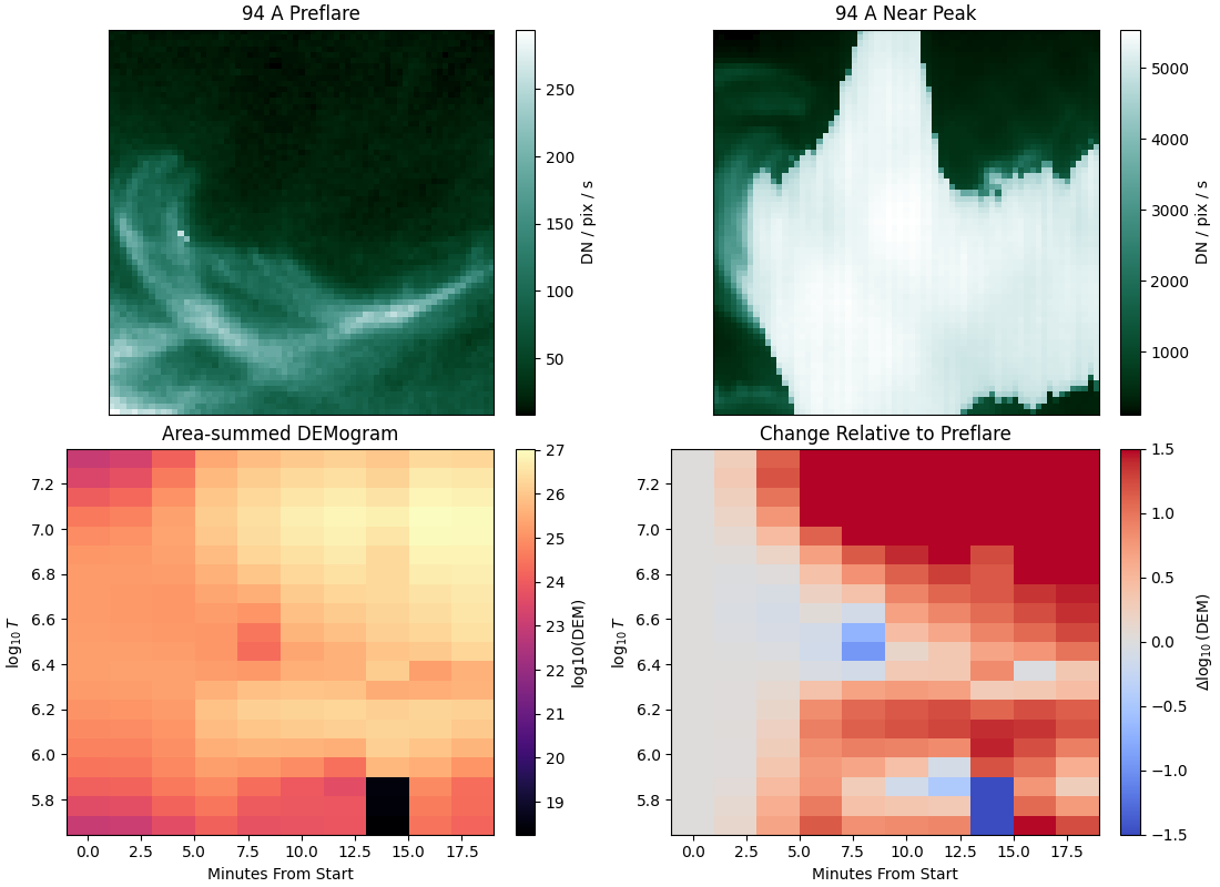
Unfortunately, as we can see in the 94 Angstrom channel, AIA is saturated during the flare and after this point DEMs become unphysical as instrument channel counts are no longer proportional to the radiation.